Tutorial: W7X VMEC Equilibria with EXTENDER
This tutorial walks the user through running the EXTENDER code for a VMEC equilibria on the W7X machine. In these runs two threads are utilized by the EXTENDER code (-np 2). The output from a VMEC run, along with tutorial files are provided here: The VMEC equilibrium output: wout_std_scp00_beta1.nc B-Field Test Points File: b_test Extender Control File: extender_in
Example 1: Calculating the fields at a point in space
In this example we run EXTENDER in order to calculate the plasma field at a series of points external to the VMEC equilibria. First let's examine where we will be evaluating the field with respect to the VMEC equilibria. The b_test points file looks like:
# Sample points file
# R    PHI     Z
 5.5   0.0    0.0
 5.6   0.0   -0.2
 5.6   0.0   -0.1
 5.6   0.0    0.0
 5.6   0.0    0.1
 5.6   0.0    0.2
 4.6   0.628   -0.2
 4.6   0.628   -0.1
 4.6   0.628    0.0
 4.6   0.628    0.1
 4.6   0.628    0.2
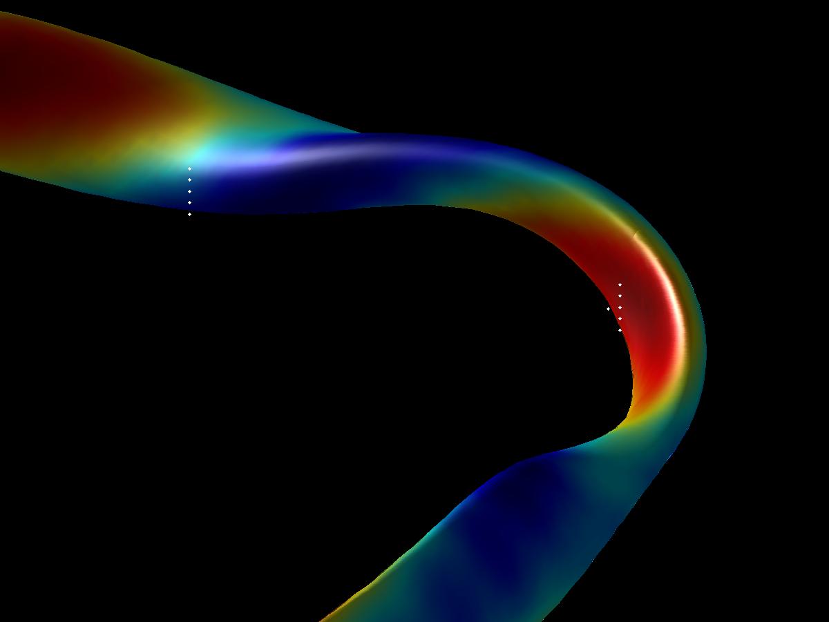
Here is a depiction of these points in space:
 The control file looks like:
nr 200   # number of radial grid points
nz 200   # number of vertical grid points
nphi 72  # number of toroidal cut planes
rmin 4.5 # optional param., can be computed autom. from boundary
rmax 6.5 # optional parameter
zmax 1.0 # optional parameter
The code is executed using the mpirun command. Here we've selected to use 2 processors (-np 2). We will be running the code using a VMEC Nyquist file (netCDF 8.47), with our control file, using 360 poloidal grid points on the surface, 72 toroidal grid points on the surface, test as our output suffix, and we wish to find our plasma field.
> mpirun -np 2 ~/bin/EXTENDER_P -vmec_nyquist wout_std_scp00_beta1.nc -i extender_in -NU 360 -NV 72 -s test -points b_test -plasmafield
persistent objects table created
reading VMEC file wout_std_scp00_beta1.nc ...
reading VmecNetcdfNyquist
persistent objects table created
reading VMEC file wout_std_scp00_beta1.nc ...
reading VmecNetcdfNyquist
entering Vmec::post_read()
entering Vmec::post_read()
Vmec::post_read completed
VMEC file wout_std_scp00_beta1.nc read successfully
reading command file
orientation = 1
generating current sheet
Vmec::post_read completed
VMEC file wout_std_scp00_beta1.nc read successfully
reading command file
orientation = 1
generating current sheet
commencing computation
pe 0 arrived at barrier
commencing computation
pe 0 arrived at barrier
>
This creates a b_test.out file which contains the magnetic field (H) information regarding the points in the b_test points file. Our output looks like:
#  i      r       phi       z       H_r       H_phi       H_z       |H|    inside
       0  5.50000000e+00  0.00000000e+00  0.00000000e+00  2.33323875e+00  1.33290897e+03 -1.66599741e+02  1.34328227e+03 0
       1  5.60000000e+00  0.00000000e+00 -2.00000000e-01 -1.77868044e+01  1.36686179e+03 -2.92511781e+02  1.39792369e+03 0
       2  5.60000000e+00  0.00000000e+00 -1.00000000e-01 -1.28263563e+01  1.42632806e+03 -1.67522929e+02  1.43618947e+03 0
       3  5.60000000e+00  0.00000000e+00  0.00000000e+00  1.91169944e+01  1.44658408e+03 -1.30659449e+02  1.45259865e+03 0
       4  5.60000000e+00  0.00000000e+00  1.00000000e-01  1.28263564e+01  1.42632806e+03 -1.67522929e+02  1.43618947e+03 0
       5  5.60000000e+00  0.00000000e+00  2.00000000e-01  1.77868044e+01  1.36686179e+03 -2.92511781e+02  1.39792369e+03 0
       6  4.60000000e+00  6.28000000e-01 -2.00000000e-01  1.47611615e+03 -1.09833561e+03 -1.79915159e+03  2.57336481e+03 0
       7  4.60000000e+00  6.28000000e-01 -1.00000000e-01  8.65399072e+02 -1.29202194e+03 -2.30594544e+03  2.78129837e+03 0
       8  4.60000000e+00  6.28000000e-01  0.00000000e+00  1.15886107e+01 -1.36780443e+03 -2.50911447e+03  2.85774013e+03 0
       9  4.60000000e+00  6.28000000e-01  1.00000000e-01 -8.54243992e+02 -1.29462806e+03 -2.30999002e+03  2.78241775e+03 0
      10  4.60000000e+00  6.28000000e-01  2.00000000e-01 -1.46828715e+03 -1.10232529e+03 -1.80566541e+03  2.57515354e+03 0
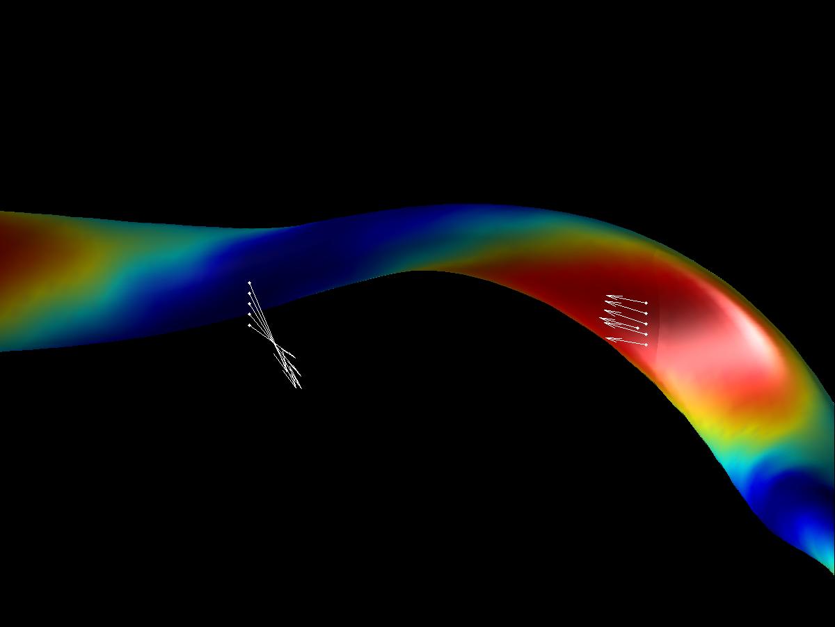
Plotting the vector field we see: